2D versus 3D Magnetotelluric Imaging
Geology & Geophysics
Magnetotelluric (MT) imaging has come a long way in the last 10 years. A decade ago, you'd have to leave a 2D inversion running on your desktop computer over night; now, it'll run on modern laptops in just 15 minutes. Similarly, a decade ago, 3D inversions were barely possible due to computational resource limitations; now, they're the industry standard.
Until somewhat recently, most MT studies (academic as well as industrial) were performed in 2D, due to the aforementioned computational limitations. 2D inversion of MT data is certainly a useful approximation in some situations; however, 3D MT inversion now makes it possible to extract more information from the data and to gain much more robust insights into what the data are telling us about subsurface conductivity structure.
In this article, we're going to take a look at some comparisons between 2D and 3D inversion of the same data. As you'll see, sometimes the 2D and 3D inversion results are similar, but sometimes they're very different, with implications for the questions you're trying to answer.
Dataset and Methodology. The dataset we're using here is shown in Figure 1 below. We inverted the full dataset in a fully 3D inversion, and we also selected four profiles of sites with which we performed 2D profile inversions and individual 3D inversions just of the profile sites. For each of the four profiles, this gives us three images to compare: the corresponding slice through the full 3D model, the slice through the 3D inversion using only the profile data, and the 2D inversion for the profile.
We won't go into the details of our inversion methodology here, but suffice to say that our approach for 2D inversions is similar to what has often been done (and still is being done to some extent) in industrial MT applications.
2D vs 3D Comparisons
Figure 1 shows a depth slice through the full 3D conductivity model derived from the full dataset. As you can see, there are several major conductivity lineaments, and we chose our four data profiles to cross these lineaments.
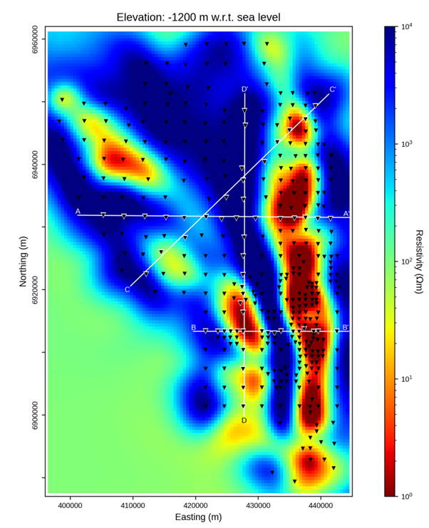
Figure 1: Depth slice through the full 3D conductivity model. Inverted black triangles denote MT sites used in the inversion. White lines denote the four profiles shown below. White halos denote sites used along the profiles.
Figures 2 through 5 below show the comparisons of the three different inversion images (full 3D, profile 3D, and 2D) along each profile.
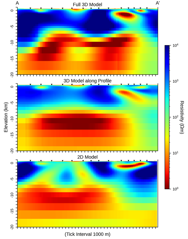
Figure 2: Comparison of three inversion images along profile A-A'.
The images along profile A-A' (Fig. 2, above) show major differences between the 2D and 3D imaging results. The full 3D and 3D profile inversions show broadly similar structures, with a resistive upper crust (<5 km depth) overlying a conductive mid crust (>5 km depth) and an isolated shallow (~2 km depth) east-dipping conductor at the right (east) end of the profile. In contrast, the 2D image shows moderately conductive channels in the upper crust (<5 km depth), and the isolated shallow conductor becomes west-dipping. These differences demonstrate the complexity of structure along this profile.
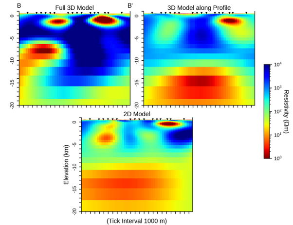
Figure 3: Comparisons of three inversion images along profile B-B'.
The images along profile B-B' (Fig. 3, above) are broadly similar between different inverse solutions, but neither the 2D inversion nor the 3D profile inversion captures the details of conductors imaged in the full 3D inversion. The 2D inversion also generally makes the shallow crust (<5 km depth) more conductive than the two 3D inversions, with an extra weakly conductive feature midway along the profile.
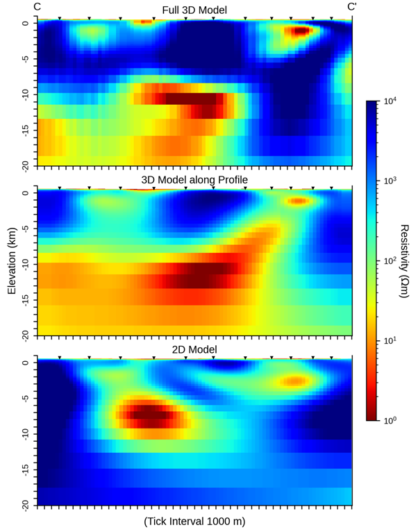
Figure 4: Comparisons of three inversion images along profile C-C'.
The images along profile C-C' (Fig. 4, above) are again broadly similar between inversions, but structural details are often markedly different in each solution. For example, all three solutions capture the shallow (~2 km) conductor on the right (northeast) side of the profile, but each solution shows a different structural attitude of that conductor to the southwest. The highly conductive mid crustal conductor (>10 km depth) is also imaged differently in the 2D solution compared to two 3D solutions.
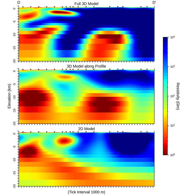
Figure 5: Comparisons of three inversion images along profile D-D'.
Finally, the images along profile D-D' are yet again broadly similar, but in detail they differ markedly. Notably, the full 3D and 3D profile inversions resolve the two separate deep (>5 km depth) conductors, whereas the 2D inversion only resolves a laterally continuous dipping conductive zone at the corresponding depths. The 3D inversions are revealing more structural information here.
Conclusions
As you can see, sometimes the 2D and 3D inversion results would lead you to similar interpretations. However, sometimes the 2D inversion results show features that are not supported by the 3D inversions (e.g., Fig. 2), and the 3D images reveal important information about our view of the subsurface.
Although 2D inversions are very useful in certain situations, we consider the 3D images to be a more robust, information-rich depiction of subsurface conductivity structure. The 2D inversions are not necessarily "wrong", but they are constrained by assumptions of 2D structure. In contrast, 3D inversions permit more degrees of freedom to, for example, place localized structures off-axis of a profile of sites, rather than directly along the profile as with 2D inversions. The 3D images are consequently able to more readily honor the requirements of the data and thereby yield different, potentially more reliable insights into subsurface structure.
Ideally, for resource exploration work, you would have access to an array of sites across a project area that could be used for a fully 3D inversion of the data. However, if you've only got MT sites along a profile, then even just running a 3D inversion on that data profile can provide new insights compared to a 2D inversion (e.g., Figs. 2, 5). The 3D profile inversion is not necessarily the most "correct" (e.g., Figs. 3, 4), but it nevertheless yields more information than 2D inversions alone. Comparing the 3D profile image to the 2D image can show you, for example, which structures are reliable and which structures you'd want to constrain with more data before attempting to drill.
If you're working with legacy MT data, these will most likely have only been inverted in 2D (or even just 1D), since that's all that could be done when they were originally collected. Today, it's trivial to re-invert legacy MT data using 3D inversion tools, and doing so can reveal much more robust insights into subsurface structure than the original 2D (or 1D) images alone.
About Us
Moombarriga Geoscience is a full-service MT and DC/IP services company. We collect and process data, and we perform inversions and interpretations -- including 3D re-inversions of legacy MT data that may have previously only been analyzed under 2D assumptions. We also provide off-the-shelf 3D re-inversion data products of legacy government geophysical reports, ready for incorporation into modern exploration programs.
Contact us today to discuss your geophysical needs!