Recent News & Projects.
The inversion of magnetotelluric (MT) data is as much an art form as it is a science. Not only does a full 3D MT inversion (which is what everyone should be doing these days!) take a lot of computational resources (we're talking supercomputers here), but it also demands a high degree of expertise from the professional performing the inversion. To get good inversion results, you really need someone who has access to good inversion tools and who really knows how to use them. The black-box approach doesn't work here! When MT is done well, the results can be spectacularly valuable to a project. When MT is done poorly, you can end up feeling like you dropped a big chunk of cash for nothing. The difference between success and failure here depends highly on the expertise of your contractor. So, to illustrate this point, let's take a look at an example of well-done MT.
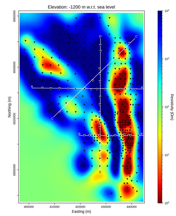
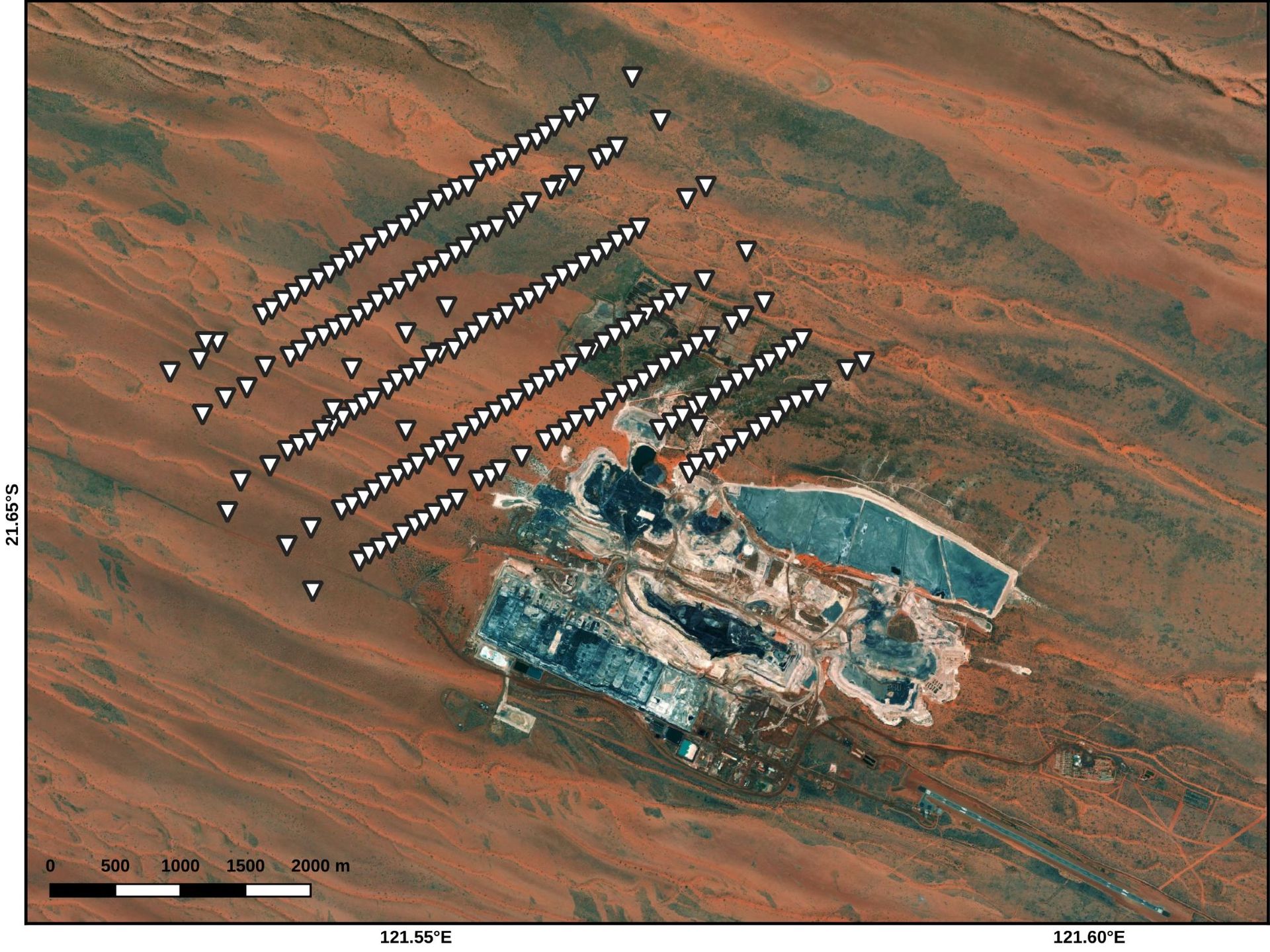
Geology & Geophysics Magnetotelluric (MT) imaging has come a long way in the last 10 years. A decade ago, you'd have to leave a 2D inversion running on your desktop computer over night; now, it'll run on modern laptops in just 15 minutes. Similarly, a decade ago, 3D inversions were barely possible due to computational resource limitations; now, they're the industry standard. Until somewhat recently, most MT studies (academic as well as industrial) were performed in 2D, due to the aforementioned computational limitations. 2D inversion of MT data is certainly a useful approximation in some situations; however, 3D MT inversion now makes it possible to extract more information from the data and to gain much more robust insights into what the data are telling us about subsurface conductivity structure. In this article, we're going to take a look at some comparisons between 2D and 3D inversion of the same data. As you'll see, sometimes the 2D and 3D inversion results are similar, but sometimes they're very different, with implications for the questions you're trying to answer. Dataset and Methodology. The dataset we're using here is shown in Figure 1 below. We inverted the full dataset in a fully 3D inversion, and we also selected four profiles of sites with which we performed 2D profile inversions and individual 3D inversions just of the profile sites. For each of the four profiles, this gives us three images to compare: the corresponding slice through the full 3D model, the slice through the 3D inversion using only the profile data, and the 2D inversion for the profile. We won't go into the details of our inversion methodology here, but suffice to say that our approach for 2D inversions is similar to what has often been done (and still is being done to some extent) in industrial MT applications. 2D vs 3D Comparisons Figure 1 shows a depth slice through the full 3D conductivity model derived from the full dataset. As you can see, there are several major conductivity lineaments, and we chose our four data profiles to cross these lineaments.