The Power of Properly Done MT
The inversion of magnetotelluric (MT) data is as much an art form as it is a science. Not only does a full 3D MT inversion (which is what everyone should be doing these days!) take a lot of computational resources (we're talking supercomputers here), but it also demands a high degree of expertise from the professional performing the inversion. To get good inversion results, you really need someone who has access to good inversion tools and who really knows how to use them. The black-box approach doesn't work here!
When MT is done well, the results can be spectacularly valuable to a project. When MT is done poorly, you can end up feeling like you dropped a big chunk of cash for nothing. The difference between success and failure here depends highly on the expertise of your contractor.
So, to illustrate this point, let's take a look at an example of well-done MT.
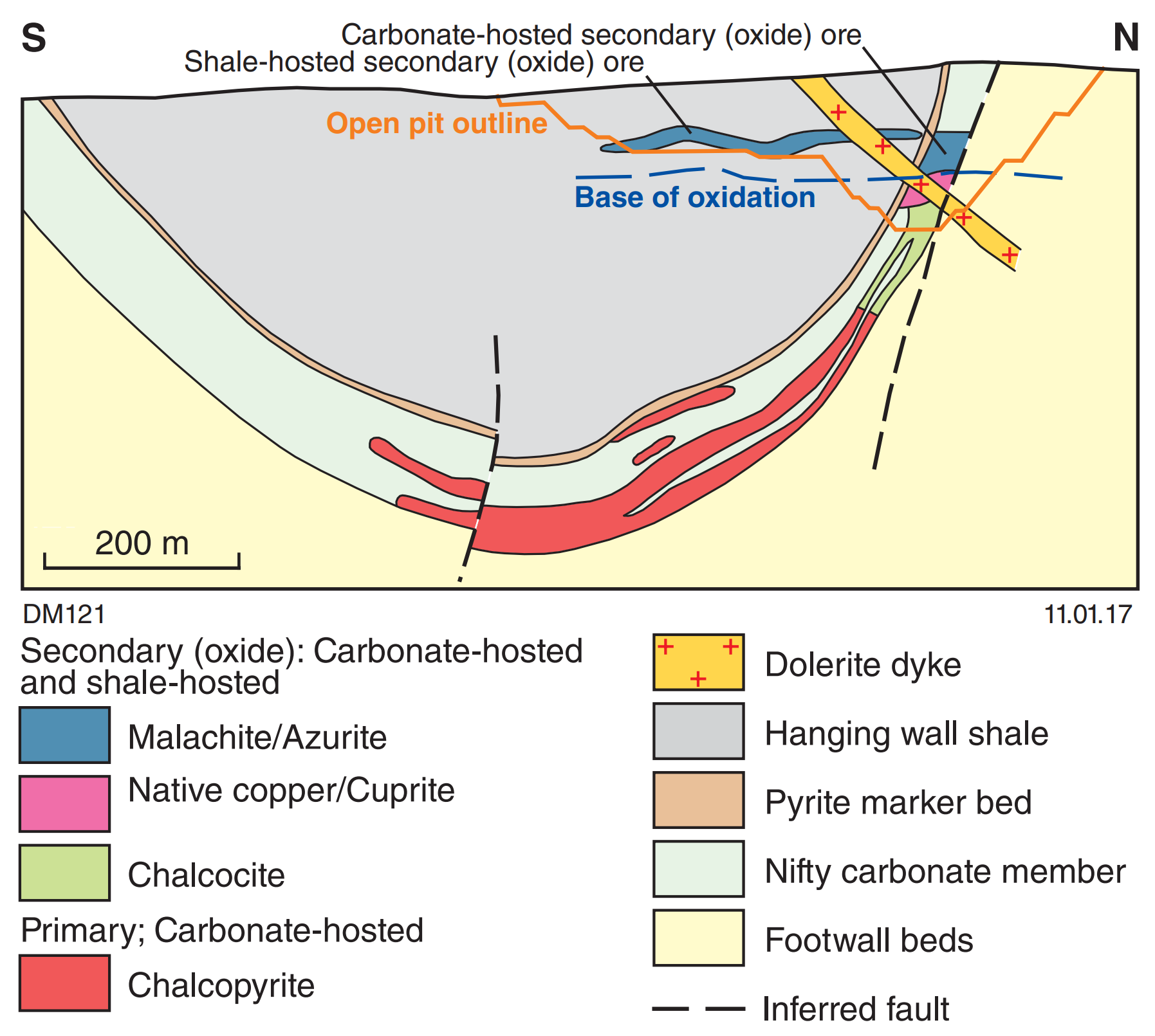
Geologic cross section through the Nifty Syncline and the Nifty deposit. From Maidment et al., 2017.
The Nifty Deposit
For this example, we're going to look at an MT dataset that was collected adjacent to the Nifty deposit, in Western Australia.
Nifty is a sediment-hosted copper deposit within the limb of a southeast-plunging syncline. The mine has largely tapped supergene and hypogene enrichment zones, but primary copper mineralization is stratabound chalcopyrite. The host rock for this mineralization is the Nifty member of the Broadhurst Formation, part of a sequence of Neoproterozoic low-grade metasedimentary rocks. The figure below shows a cross section through the Nifty Syncline and the Nifty deposit.
The Broadhurst Formation can be generally divided into three broad sub-units: the lower and upper portions largely consist of carbonaceous and sulfidic pelitic rocks with interbedded carbonates, and the middle portion broadly consists of psammitic rocks (Porter, 2017). The Nifty member, which hosts the Nifty deposit, is in the lower part of the upper pelitic sub-unit.
Due to their carbonaceous and sulfidic nature, these upper and lower sub-units are highly electrically conductive. Geophysically, they contrast strongly with the electrically resistive psammitic rocks that constitute the middle sub-unit of the Broadhurst Formation and the underlying Coolbro Formation.
So, let's say you want to look for additional mineralized zones within the Nifty Syncline, away from the Nifty deposit. To do this, you would most likely want to map the structure and extent of the syncline. Fortunately, the electrically conductive units within the Nifty Syncline make excellent geophysical marker horizons for accomplishing these purposes. The Syncline, however, is covered by conductive overburden, and it also extends deep (>1 km). Due to these factors, MT is an excellent choice for geophysical imaging of the Nifty Syncline.
The Nifty Dataset
The map below shows the MT dataset that we collected over the Nifty Syncline, to the northwest of the Nifty deposit itself. These data were collected in 2014 with Phoenix MT instruments.
Inversions Done Well
We've performed 3D inversion of the Nifty dataset using CGG's Geotools platform and their RLM3D inversion code. Images of our inversion results are shown below. As you can see, the Nifty Syncline is imaged exceptionally well. The conductivity images show the textbook map pattern of a southeast-plunging syncline.
Clearly, there is exploration value here: we can see the structure of the Nifty Syncline, as defined by the conductive marker beds, and we can trace out those key markers. The ore-bearing Nifty member occurs in the lower part of the upper pelitic sub-unit of the Broadhurst Formation, and we can see spatially where that is located in these conductivity images.
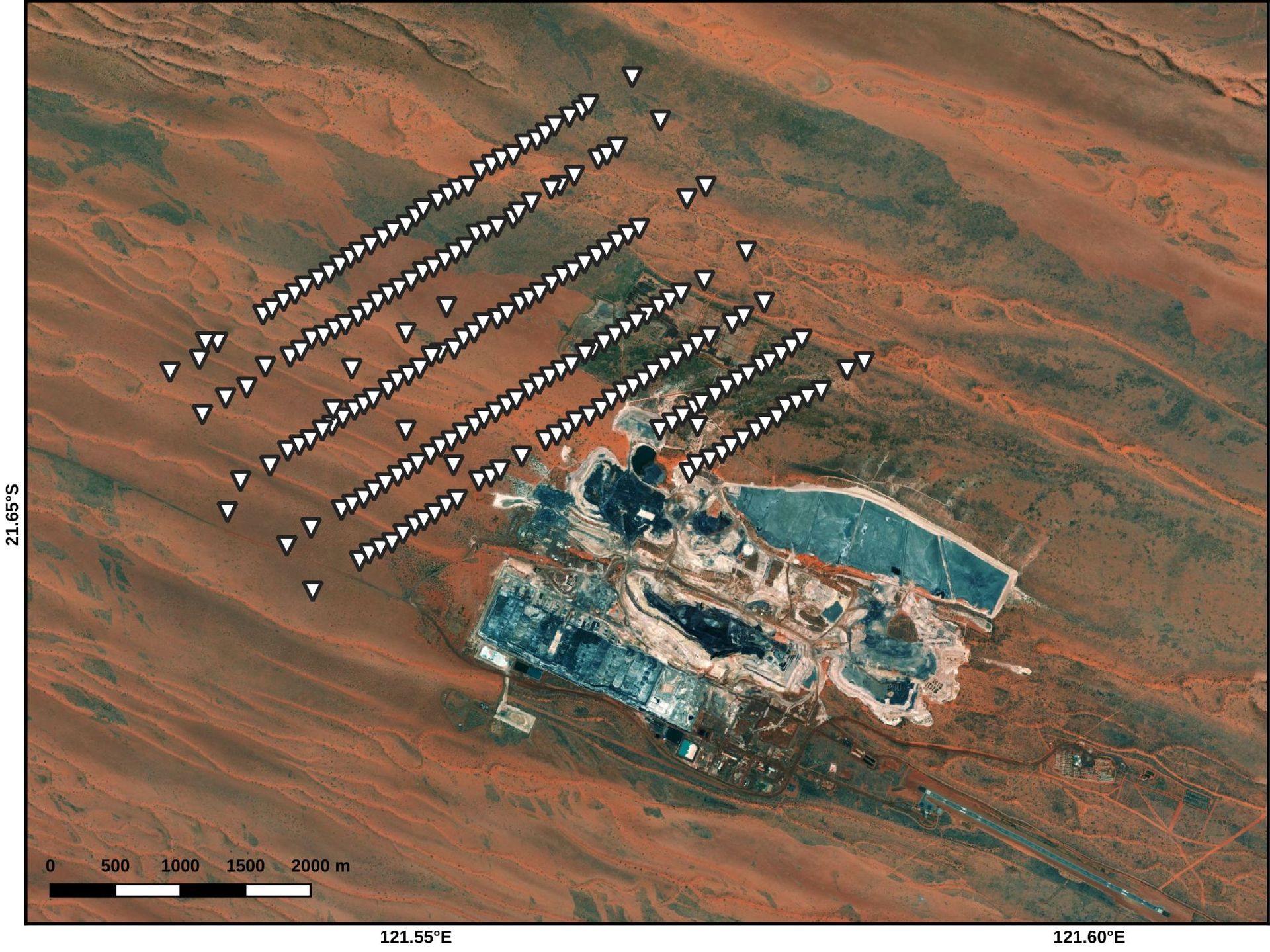
AMT/MT sites (white inverted triangles) collected by Moombarriga Geoscience to the northwest of the Nifty deposit, over the Nifty Syncline.
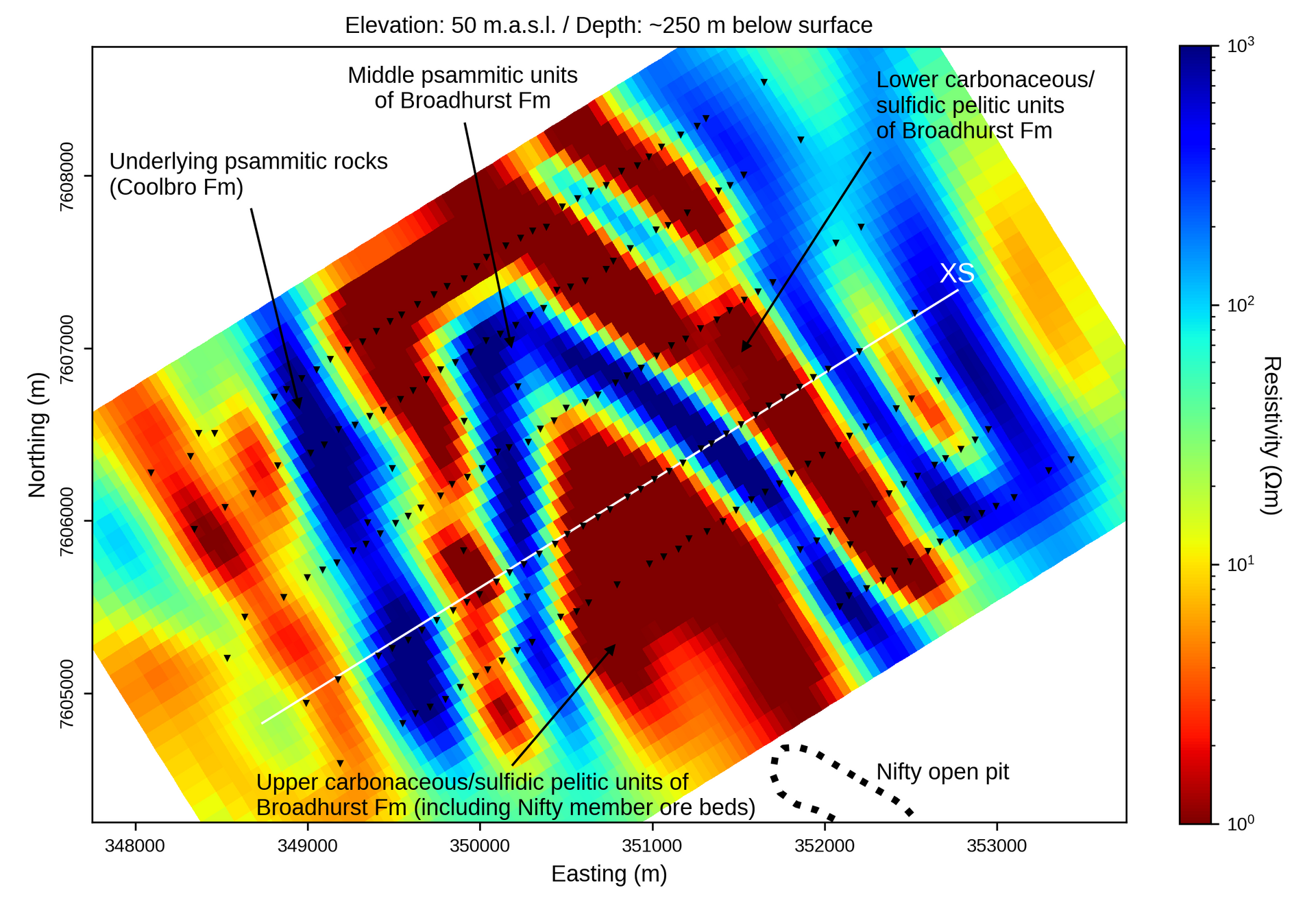
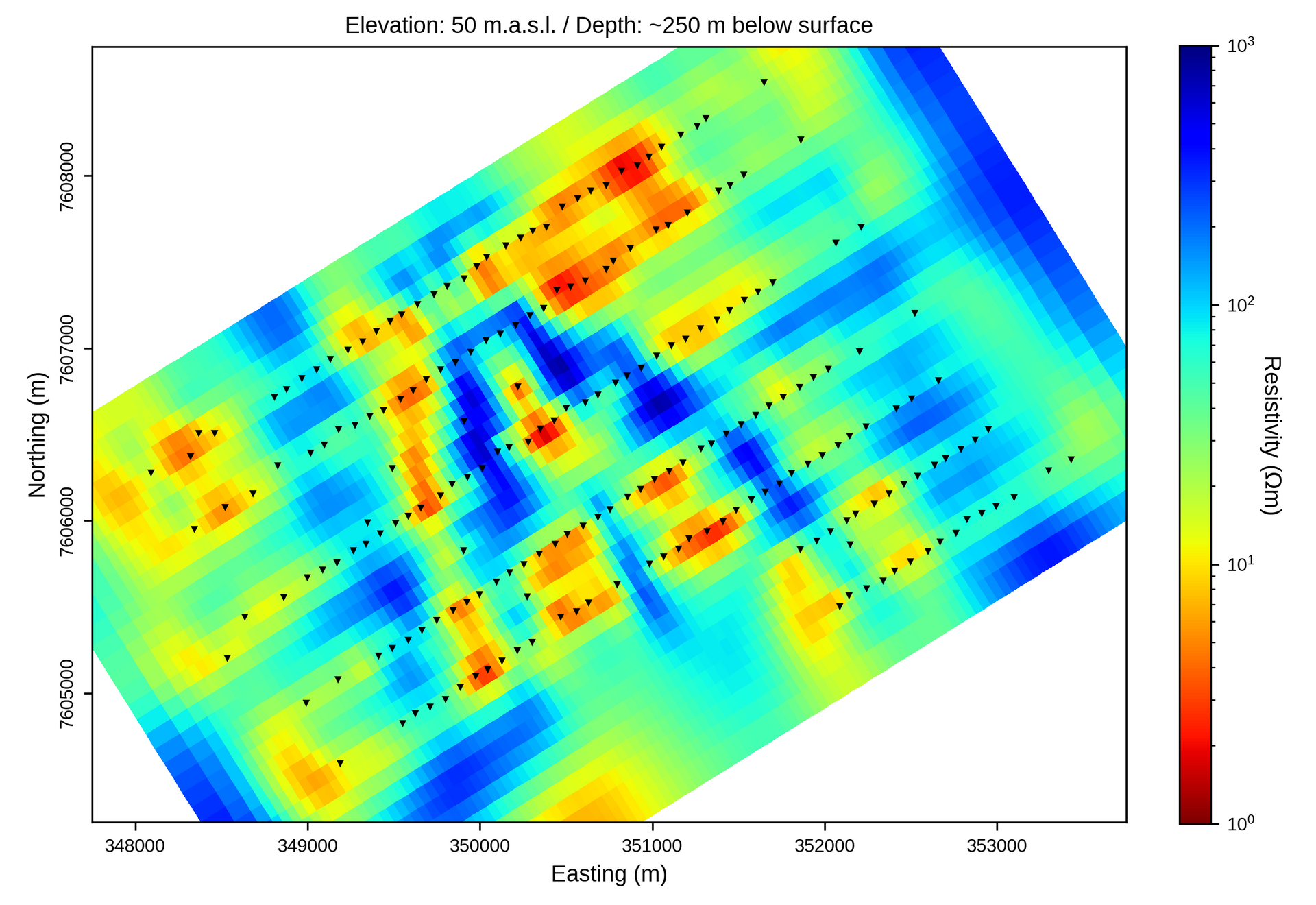
Slice at an elevation of 50 m above sea level (~250 m below the surface) through the electrical conductivity model developed for the Nifty dataset. Note that warm colors denote low resistivity (high conductivity) values.
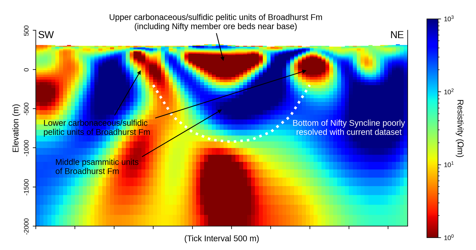
Cross section through the electrical conductivity model developed for the Nifty dataset. Cross section location is shown with the white "XS" line in the previous figure.
For those of you curious about data misfit, we can assure you that this conductivity models fits and explains the data quite well!
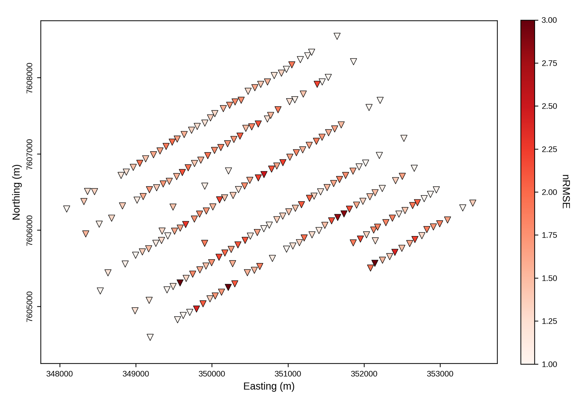
Normalized root-mean-square (nRMSE) site-by-site misfit for the conductivity images shown above.
Now, the value delivered with these images was unlocked because we know how to get good inversion results from the tools we have on-hand. Improperly setting even one inversion parameter can result in complete destruction of that value. This is demonstrated by the image below, which was derived by slightly changing one set of regularization parameters in the inversion.
Depth slice (at 50 m above sea level / ~250 m below the surface) through a "bad" conductivity model derived from the Nifty dataset; the only difference from the depth slice above is a change in regularization.
About Us
Moombarriga Geoscience is a full-service MT and DC/IP services company. We collect and process data, and we perform inversions and interpretations. Contact us today to discuss your geophysical needs!
References
D.W. Maidment, D.L. Huston, and T. Beardsmore (2017). Paterson Orogen geology and metallogeny. In G.N. Phillips (ed), Australian Ore Deposits, The Australasian Institute of Mining and Metallurgy, Monograph 32.
T.M. Porter (2017). Nifty and Maroochydore copper deposits. In G.N. Phillips (ed), Australian Ore Deposits, The Australasian Institute of Mining and Metallurgy, Monograph 32.